Survival Analysis Basics: Time-to-Event Data Explained

Meta Title: Survival Analysis Basics: Time-to-Event Data Explained (2026 Guide)

Meta Description: Learn survival analysis basics, from censoring to Kaplan-Meier curves. A clear guide to time-to-event data for researchers and data analysts.

Slug: survival-analysis-basics-time-to-event-data

Introduction

Survival analysis answers a fundamental question: how long until something happens?

Despite the name, survival analysis isn’t just about death. It’s used whenever you’re interested in the time until an event occurs whether that’s a patient recovering from illness, a machine failing, or a customer canceling a subscription .

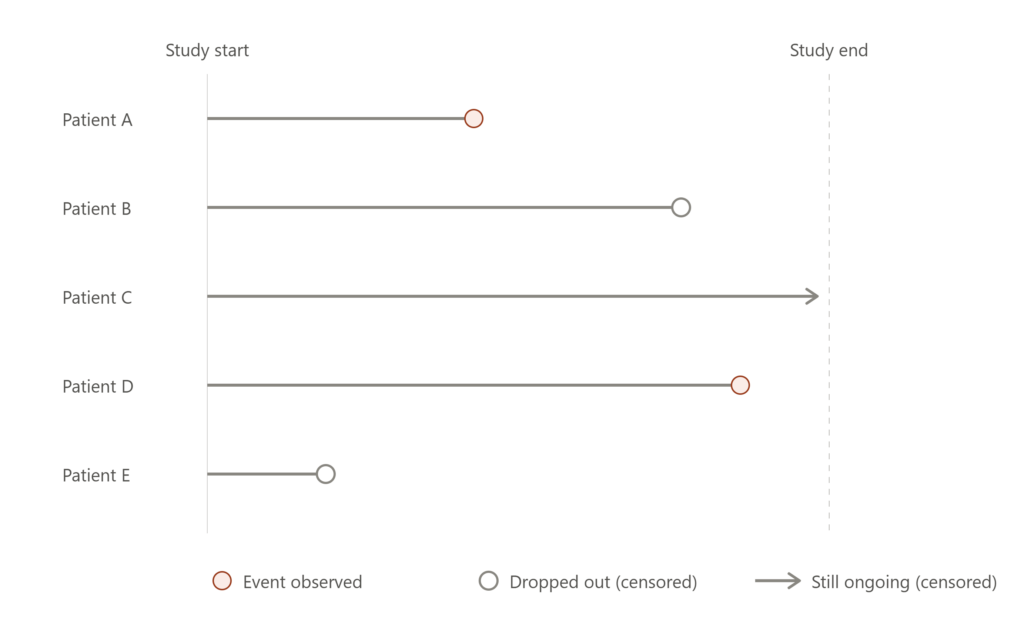
The challenge? You rarely observe every event. Some patients drop out of studies. Some machines are still running when the study ends. This incomplete information is what makes time-to-event data special and what makes standard statistical methods unsuitable .

This guide covers the essential concepts: what makes time-to-event data unique, why censoring matters, and the core tools like Kaplan-Meier curves and Cox regression.

What Makes Time-to-Event Data Different?

Time-to-event data, also called survival data, consists of two pieces of information for each subject: the time under observation and whether the event occurred .

What distinguishes this from ordinary regression is that the outcome isn’t just a number it’s a when. And that “when” is often incompletely observed.

Consider a clinical trial tracking time to disease recurrence. At the end of the study:

Some patients experienced the event (recurrence occurred)
Some are still event-free (recurrence hasn’t happened yet)
Some dropped out (lost to follow-up)

You can’t simply calculate an average survival time because you don’t know when the event-free patients will eventually have their event. They might remain event-free for years or the event might occur the day after the study closes .

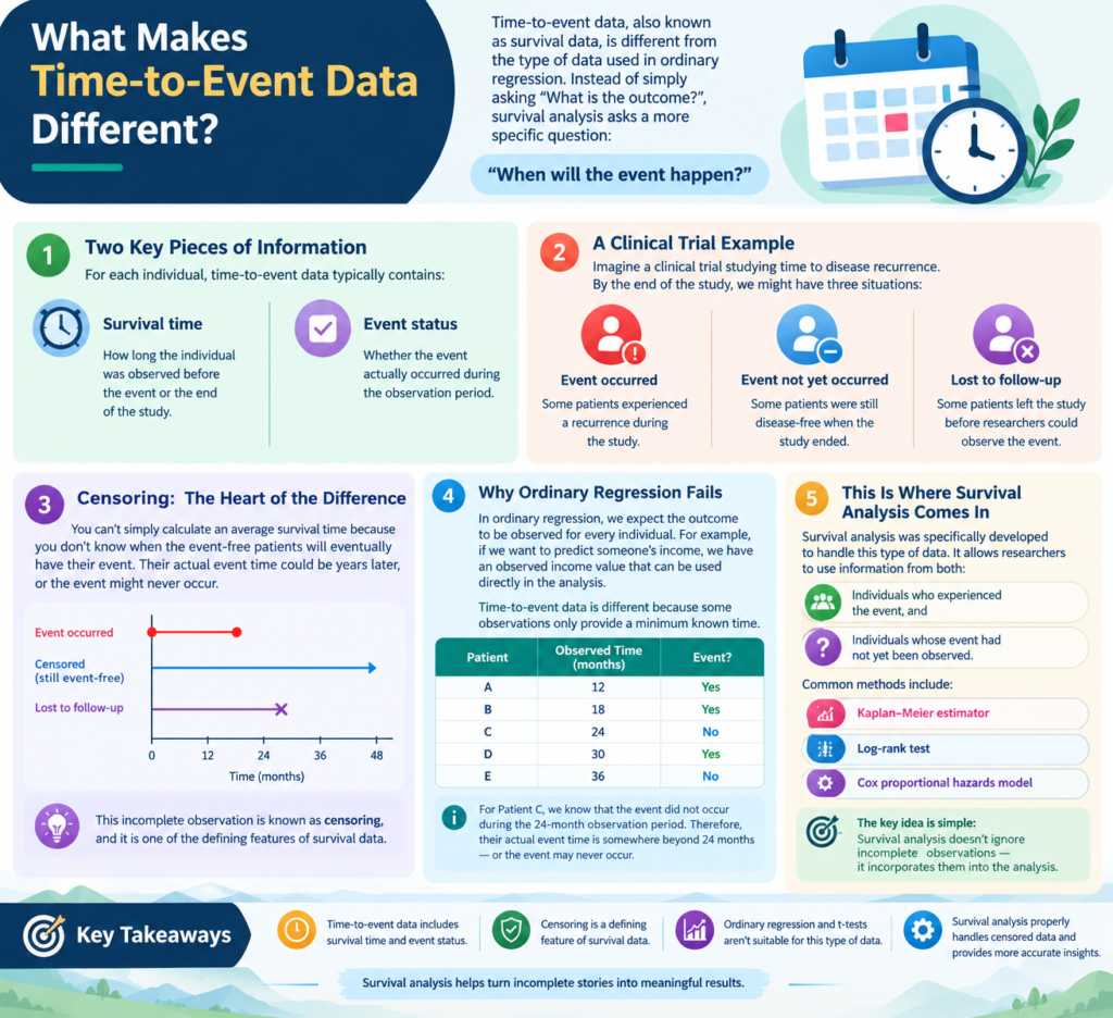
Standard statistical tests like t-tests or linear regression fail here because they require complete outcome data. Survival analysis was developed specifically to handle this incompleteness.

The Censoring Problem

Censoring is the defining feature of time-to-event data. It occurs when you have partial information about a subject’s survival time—you know the event hasn’t happened yet, but you don’t know when it will .

Right Censoring: The Most Common Type

Right censoring happens when the event occurs after the observation period ends. You know the true survival time is longer than the observed time, but you don’t know by how much .

Common causes include:

The study ends before the event occurs
The patient withdraws or is lost to follow-up
The patient dies from an unrelated cause

The key assumption is non-informative censoring: the reason for censoring is unrelated to the likelihood of the event occurring. If patients drop out because they’re getting sicker (and thus more likely to have the event), your results will be biased .

Other Censoring Types

Left censoring: The event occurred before observation began, but the exact time is unknown
Interval censoring: The event occurred between two time points, but the exact time is unknown

Right censoring dominates most applications, especially when death is the outcome of interest.

The Survival Function: S(t)

The survival function is the probability that a subject survives beyond a given time point. Formally, if T is the time to event, then:

S(t) = P(T > t)

This function starts at 1 (everyone is alive at time zero) and decreases toward 0 as time progresses .

The survival curve is simply a plot of S(t) against time. It’s a step function that drops at each event time, with the size of each drop reflecting how many subjects experienced the event at that point.

In plain language: If S(5 years) = 0.70, that means 70% of subjects survived past 5 years. Or equivalently, 30% experienced the event within 5 years .

The Hazard Function: h(t)

While the survival function focuses on not having the event, the hazard function describes the rate at which events occur among those still at risk.

Think of the hazard as the “instantaneous risk” of the event at time t, given survival up to that point .

h(t) = probability of event in the next instant, given survival until t

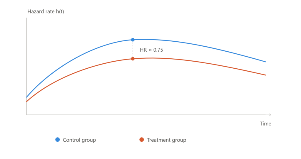
The hazard function is central to regression modeling. When you see a hazard ratio (HR), it’s comparing the hazard rates between two groups:

HR = 1: No difference in hazard between groups
HR > 1: Higher hazard (faster time to event) in the treatment/exposed group
HR < 1: Lower hazard (slower time to event), suggesting a protective effect

An HR of 0.75 means the treatment group has 25% lower hazard at any given time point—they’re experiencing the event at a slower rate.

Kaplan-Meier Estimator: The Survival Curve

The Kaplan-Meier estimator (also called the product-limit estimator) is the standard nonparametric method for estimating survival curves. It makes no assumptions about the underlying distribution of survival times .

The KM method calculates survival probabilities at each event time by:

Ordering all event times from shortest to longest
At each event time, computing the proportion of subjects at risk who experience the event
Multiplying these proportions cumulatively

The result is a step-function curve with drops at each event time. Censored observations are typically marked with tick marks on the curve .

Key advantage: The KM estimator uses information from censored subjects up until their censoring time. A patient censored at 6 months contributes to survival estimates for all time points before 6 months—we know they survived at least that long .

Comparing Curves: The Log-Rank Test

When you have two or more groups (e.g., treatment vs. control), you can plot separate Kaplan-Meier curves and compare them using the log-rank test.

The log-rank test evaluates whether the survival distributions differ significantly between groups. It’s the standard hypothesis test for comparing survival curves .

Cox Proportional Hazards Model

While Kaplan-Meier curves show whether groups differ, the Cox proportional hazards model quantifies how much different factors affect survival time .

The Cox model is semiparametric: it doesn’t assume a specific distribution for survival times, but it does assume that covariates have a multiplicative effect on the hazard that remains constant over time (the proportional hazards assumption) .

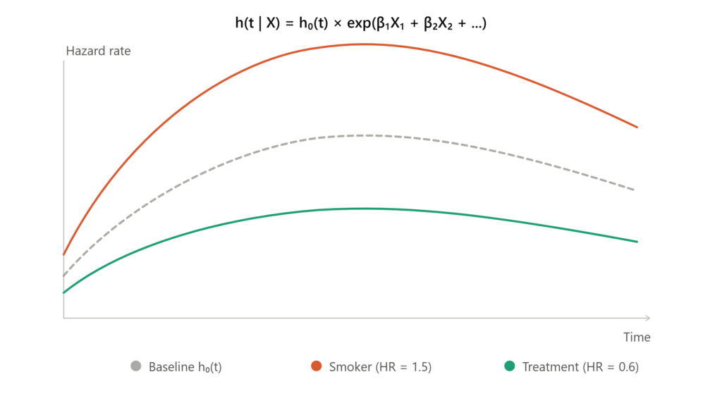
The model produces hazard ratios for each covariate, which you can interpret directly:

A hazard ratio of 1.5 for smoking means smokers have 50% higher hazard at any time point
A hazard ratio of 0.6 for a treatment means the treatment reduces hazard by 40%

This makes Cox regression particularly valuable for identifying risk factors and evaluating interventions .

Practical Example: Kidney Transplant Data

To illustrate these concepts, consider a dataset tracking time to kidney transplant failure. Some patients experience transplant failure during follow-up; others are still functioning at study end (censored).

A Kaplan-Meier curve would show the probability of transplant survival over time. The Cox model could estimate hazard ratios for factors like donor age, recipient age, and HLA mismatch revealing which factors accelerate or delay failure.

Most statistical software handles these methods routinely. In R, the survival package is standard; in Python, the lifelines library provides similar functionality .

Common Pitfalls to Avoid

1. Ignoring censoring. Simply analyzing observed event times as if they were complete data produces biased results. Always use survival-specific methods.

2. Violating proportional hazards. The Cox model assumes hazard ratios are constant over time. If the effect of a treatment diminishes (or grows) over time, this assumption is violated. Test with Schoenfeld residuals.

3. Informative censoring. If censoring is related to prognosis, standard methods produce biased estimates. Document reasons for dropout and consider sensitivity analyses .

4. Misinterpreting hazard ratios. HR ≠ risk ratio, though they’re often interpreted similarly. The HR is a ratio of instantaneous hazards, not cumulative risks.

Key Takeaways

Survival analysis provides the statistical framework for answering “how long until?” questions when data are incomplete due to censoring.

Time-to-event data records both time and event status, with censoring creating incomplete observations
Censoring is the defining challenge—right censoring is most common
The survival function S(t) describes the probability of remaining event-free over time
The hazard function h(t) describes the instantaneous event rate among those at risk
Kaplan-Meier curves estimate survival nonparametrically
The Cox model quantifies covariate effects via hazard ratios

Whether you’re analyzing clinical trial data, customer churn, or equipment failure, these tools help you extract meaningful insights from time-to-event data.

Suggested Internal Links:

Kaplan-Meier Curves Explained: A Visual Guide
Cox Regression: Interpreting Hazard Ratios
R vs. Python for Survival Analysis

Suggested External Links:

survival R package documentation
lifelines Python library documentation