
How to Detect and Fix It (Step-by-Step)
There is a peculiar kind of frustration in regression modelling when your model looks perfectly fine on the surface, but nothing quite adds up underneath. Coefficients flip signs when you add a new variable. A predictor that theory says should matter shows up non-significant. Your standard errors are suspiciously large. If any of this sounds familiar, multicollinearity is likely the culprit.
This guide walks you through what it is, how to catch it, and most importantly how to deal with it.
Part 1 — What Exactly Is Multicollinearity?
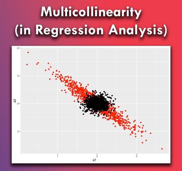
Multicollinearity occurs when two or more independent variables in your regression model are highly correlated with each other. In plain language, they are measuring overlapping things. When this happens, the model struggles to separate out the individual effect of each predictor. It cannot tell which variable is doing the work, so it inflates the standard errors and makes coefficients unreliable.
Imagine trying to figure out which twin ate the last biscuit, when they were both in the kitchen at the same time. That is multicollinearity. Your model simply cannot tell the two apart.
Important: Multicollinearity does not reduce your model’s overall predictive power. R-squared and F-statistic are largely unaffected. What it destroys is your ability to interpret individual coefficients. And for thesis work, interpretation is everything.
Part 2 — How to Detect Multicollinearity
There are three reliable ways to detect multicollinearity, ranging from quick visual checks to formal statistical tests. Use all three as they catch different things.
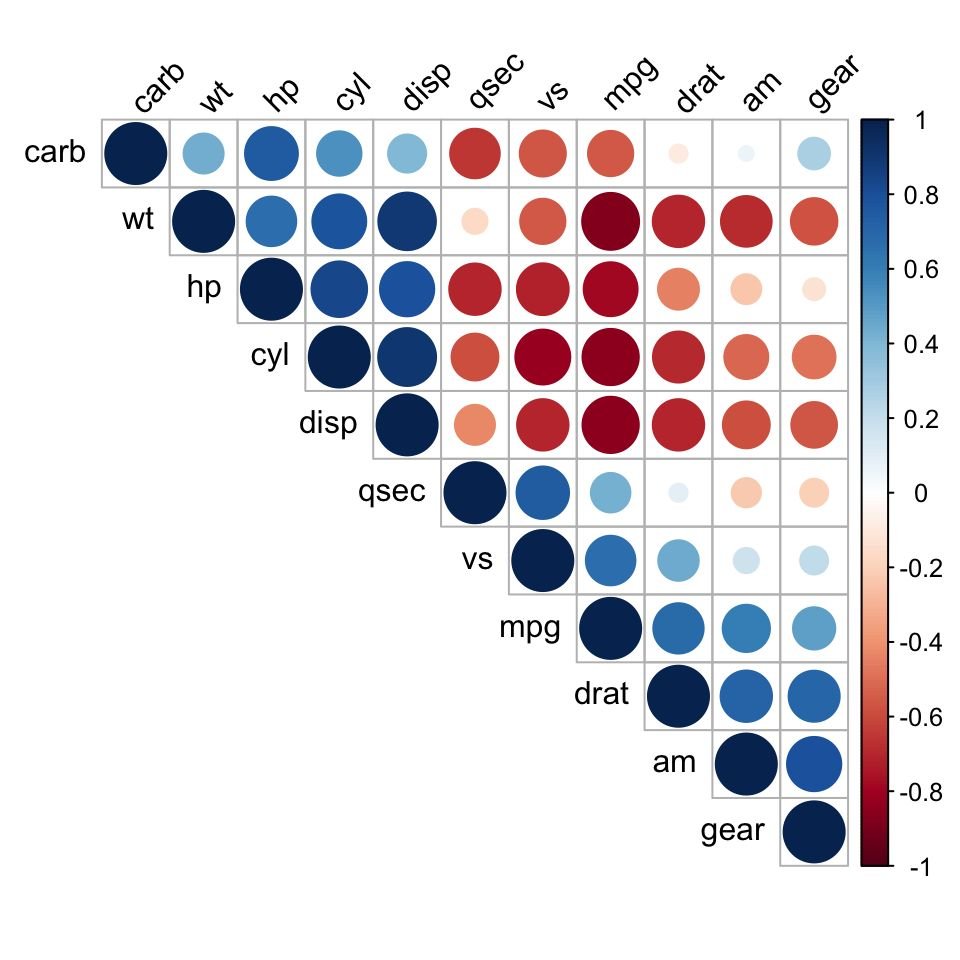
Method 1: Correlation Matrix
Start with the simplest check. Run a pairwise correlation matrix between all your independent variables. Any correlation above 0.80 is a red flag that deserves closer examination.
In SPSS: Analyze > Correlate > Bivariate
In R:
cor(data[, c(‘var1’, ‘var2’, ‘var3’, ‘var4’)])
In Stata:
correlate var1 var2 var3 var4
Note: A correlation matrix only catches pairwise collinearity. It can miss cases where three or more variables combine to create multicollinearity. Never rely on it alone.
Method 2: Variance Inflation Factor (VIF)
VIF is the gold standard test for multicollinearity. It measures how much the variance of a regression coefficient is inflated due to its correlation with other predictors. A VIF of 1 means no inflation at all. As VIF climbs, your coefficient estimates become increasingly unstable.
In SPSS: Analyze > Regression > Linear > Statistics > Collinearity diagnostics
In R:
library(car)
vif(model)
In Stata:
estat vif
Use the table below to interpret your VIF scores:
| VIF Value | Tolerance | Interpretation | Action Needed? |
| 1.0 – 2.0 | 0.50 – 1.00 | No multicollinearity | None required |
| 2.0 – 5.0 | 0.20 – 0.50 | Moderate – monitor | Review your model |
| 5.0 – 10.0 | 0.10 – 0.20 | High – concern | Take action |
| Above 10.0 | Below 0.10 | Severe | Must fix before interpreting |
Method 3: Tolerance Values
Tolerance is simply the inverse of VIF (Tolerance = 1 / VIF). Most statistical software reports both. A tolerance below 0.10 indicates that over 90% of the variance in that predictor is explained by the other predictors. That is a serious problem.
Part 3 — How to Fix Multicollinearity (5 Proven Solutions)
Once you have confirmed multicollinearity, the fix depends on your data, your sample size, and what your research question actually requires.
Fix 1: Remove One of the Correlated Variables
The most straightforward solution. If two variables are measuring nearly the same thing, keeping both adds noise without adding insight. Drop the one that is theoretically weaker or less central to your research question.
When to use: When you have two highly correlated predictors and theory supports prioritising one over the other.
Fix 2: Combine Variables into a Composite
If the correlated variables are theoretically related, consider combining them. You can average them, sum them, or use factor analysis or PCA to create a single composite variable that captures the shared variance without the redundancy.
When to use: When correlated variables represent facets of the same underlying construct such as income and wealth, or anxiety and stress.
In R:
data$composite <- (data$var1 + data$var2) / 2
Fix 3: Center Your Variables
Mean-centering (subtracting the mean from each variable) can reduce multicollinearity, particularly in models that include interaction terms or polynomial terms. It does not eliminate structural multicollinearity but helps with incidental collinearity caused by scaling.
In R:
data$var1_c <- scale(data$var1, center = TRUE, scale = FALSE)
Fix 4: Ridge Regression
Ridge regression is a modified version of OLS that adds a small penalty to the size of coefficients, shrinking them slightly to reduce variance. It produces biased estimates but those estimates are far more stable than OLS under multicollinearity. This is particularly useful when you need to keep all your predictors in the model for theoretical reasons.
When to use: When dropping variables is not theoretically justified and your VIF scores are consistently above 5 to 10.
In R:
library(glmnet)
ridge_model <- glmnet(x, y, alpha = 0)
Fix 5: Collect More Data
Multicollinearity is partly a sample size problem. With more observations, the model has more information to distinguish between correlated predictors. If your dataset is small and multicollinearity is high, increasing your sample can meaningfully reduce VIF scores.
When to use: When your sample is genuinely small and data collection is feasible.
Part 4 — How to Report It in Your Thesis
Whether or not you fix multicollinearity, you must report it transparently. Reviewers and examiners will check for this. Here is a clean way to report VIF results in your methodology section:
Prior to interpretation, multicollinearity was assessed using Variance Inflation Factors (VIF). All predictors returned VIF values below 5 (range: 1.12 to 3.87), and tolerance values above 0.10, indicating that multicollinearity did not pose a significant threat to the stability of the regression coefficients.
If you did find and address multicollinearity, state what you found, what you did about it, and why that decision was justified given your research context.
Conclusion
Multicollinearity is one of those problems that hides in plain sight. Your model keeps running, your R-squared looks respectable, and nothing obviously breaks until you try to interpret your coefficients and the story stops making sense.
Run your VIF scores before you write a single word of your results section. It takes five minutes and it could save you from defending a fundamentally flawed interpretation in front of your thesis committee.