Five Essential Guides for Students, Researchers & Business Analysts

A comprehensive deep dive into the most common mistakes, methods, and misconceptions in statistical hypothesis testing

CONTENTS

1.  p-Value Misinterpretation: The #1 Mistake Students Make in Thesis Writing

2.  t-Test vs ANOVA: Which One Should You Use and When?

3.  Type I and Type II Errors Explained with Real Business Examples

4.  Why Your Hypothesis is Getting Rejected: Common Testing Mistakes

5.  One-Tailed vs Two-Tailed Tests: A Simple Decision Guide

p-Value Misinterpretation: The #1 Mistake Students Make in Thesis Writing

Picture this: You have spent six months collecting data, running surveys, and wrestling with SPSS at 2 a.m. You finally run your analysis and the output reads p = 0.03. Your heart leaps. You type into your thesis conclusion: “The results are statistically significant, proving that my hypothesis is correct.”

Your supervisor returns the draft covered in red ink.

What went wrong? You fell into the single most common statistical trap in academic writing — misinterpreting what a p-value actually means. And you are in very good company. Studies have found that a majority of published researchers make the same error.

So What Does a p-Value Actually Mean?

The p-value measures the probability of obtaining results at least as extreme as the observed data, assuming the null hypothesis is true. Read that sentence again slowly. It is easy to skim over, and yet those seventeen words contain the entire source of confusion.

p-value = P(data | H₀ is true) — NOT — P(H₀ is true | data)

That distinction matters enormously. The p-value tells you how surprising your data would be in a world where the null hypothesis holds. It does not tell you the probability that the null hypothesis is false, nor does it measure the probability that your findings are real.

The Five Most Dangerous Misinterpretations

Mistake 1: “p < 0.05 proves my hypothesis is correct”

Statistical significance is not the same as proof. A small p-value tells you that your data would be unusual if the null hypothesis were true. It does not confirm that your alternative hypothesis is correct. There could be confounders, measurement errors, or simply the luck of sampling.

Mistake 2: “p = 0.06 means my result is not real”

The 0.05 threshold is a convention, not a law of nature. Ronald Fisher, who popularised the 0.05 cutoff in the 1920s, never intended it to become a rigid binary gate. A p-value of 0.06 and a p-value of 0.04 are practically indistinguishable in terms of evidence strength. Treating them as fundamentally different is known as the “bright line” fallacy.

Mistake 3: “A smaller p-value means a larger effect”

p-values are heavily influenced by sample size. With a large enough sample, even a trivially small difference — one that has zero real-world importance — will produce a p-value of 0.0001. Always pair your p-value with an effect size measure such as Cohen’s d, eta-squared, or odds ratios.

Mistake 4: “p > 0.05 means the null hypothesis is true”

Failing to reject the null is not the same as accepting it. A non-significant result could mean the effect does not exist, or it could mean your study lacked the statistical power to detect it. These are entirely different conclusions, and conflating them has derailed many a research career.

Mistake 5: “My p-value of 0.03 means there is a 3% chance I am wrong”

This might be the most seductive misreading. The p-value says nothing about the probability that your specific conclusion is an error. That probability depends on your prior beliefs, the base rate of true effects in your field, and publication bias — none of which appear in the p-value calculation.

What You Should Write Instead

Here is the good news: fixing p-value language in your thesis is straightforward once you know the correct framing. Compare these two phrasings:

Wrong: “The p-value of 0.03 proves that the new teaching method significantly improves test scores.”  Correct: “The analysis yielded p = 0.03, indicating that, assuming no true effect exists, there is a 3% probability of observing a difference this large or larger by chance alone. Combined with a moderate effect size (Cohen’s d = 0.45, 95% CI [0.12, 0.78]), these results are consistent with a meaningful improvement in test scores.”

The APA Fix: Reporting Standards That Protect You

The American Psychological Association’s 7th edition guidelines now require researchers to report exact p-values (not just “p < 0.05”), effect sizes, and confidence intervals. Following APA style is not just about formatting — it is about providing enough information for readers to evaluate your findings independently.

• Always report the exact p-value: p = 0.034, not p < 0.05
• Include effect size measures alongside every significance test
• Report 95% confidence intervals for your key estimates
• State clearly whether your test was one-tailed or two-tailed and why

⚡ Key Takeaway:  A p-value without an effect size is like a map without a scale. Technically accurate, practically useless.

The Bigger Picture: Why This Matters Beyond Thesis Marks

p-value misinterpretation is not merely an academic nuisance. It sits at the heart of the replication crisis — the discovery that a disturbing proportion of landmark findings in psychology, medicine, and economics cannot be reproduced. When researchers treat p < 0.05 as binary proof, they publish confidently on fragile ground.

In your own work, the goal is not to achieve statistical significance. The goal is to honestly characterise the evidence your data provides. Sometimes that evidence is compelling. Sometimes it is weak. Both outcomes advance knowledge when communicated with precision.

t-Test vs ANOVA: Which One Should You Use and When?

Published in Statistics Demystified  •  10 min read

You are comparing group means. The question sounds simple. Yet choosing between a t-test and an ANOVA trips up students at every level, from undergraduates to doctoral candidates. The decision matters: choose the wrong test and your results are either invalid or needlessly weak.

Let us cut through the confusion with a clear framework.

The Core Distinction in One Sentence

Use a t-test when comparing two means. Use ANOVA when comparing three or more means simultaneously.

That is the foundational rule. But as with most things in statistics, the full picture has nuance worth understanding.

The t-Test: Three Flavours, One Purpose

Independent Samples t-Test

This is the workhorse of between-group comparison. Use it when you have two separate groups — for example, students who received tutoring versus those who did not — and you want to know if their average scores differ.

Requirements: The two groups must be independent (no overlap in membership), each group should be approximately normally distributed, and the variances of the two groups should be similar (homogeneity of variance). When variances differ substantially, use Welch’s t-test instead, which adjusts the degrees of freedom accordingly.

Paired Samples t-Test

When the same participants are measured twice — before and after an intervention, or under two different conditions — you have paired data. The paired t-test accounts for the correlation between measurements from the same individual, giving you more statistical power than treating them as independent.

Classic use case: testing whether blood pressure differs before and after a medication trial in the same group of patients.

One-Sample t-Test

Occasionally you want to compare a sample mean against a known population value or a theoretical benchmark. If a factory claims its bolts are 10mm in diameter and you measure a batch, the one-sample t-test tells you whether your sample departs meaningfully from that specification.

ANOVA: When Two Groups Are Not Enough

Suppose you want to compare test performance across three teaching methods: traditional lecture, flipped classroom, and online self-study. You have three group means. Could you just run three separate t-tests — Method A vs B, A vs C, B vs C — and be done with it?

You could. But you should not. Here is why.

Each t-test carries a 5% false-positive risk (assuming alpha = 0.05). Running three tests inflates your overall Type I error rate to approximately 14.3%. With ten comparisons, it exceeds 40%. This is the multiple comparisons problem, and ANOVA is the solution.

ANOVA tests all groups simultaneously in a single omnibus test. By pooling variance information across groups, it maintains your chosen alpha level regardless of how many groups you have.

One-Way vs Two-Way ANOVA

One-Way ANOVA

Used when you have one independent variable (factor) with three or more levels. Teaching method, drug dosage, or geographic region are typical single factors. The F-statistic compares the variance between groups to the variance within groups. A large F suggests the group differences are unlikely to be noise.

Two-Way ANOVA

When you have two independent variables and want to understand both their individual effects (main effects) and whether they influence each other (interaction effects), you move to two-way ANOVA. For example: does score differ by teaching method AND by student gender, and does gender moderate the effectiveness of different teaching methods?

The interaction term is often the most interesting finding. It reveals that a treatment works differently depending on who receives it — a discovery that a series of t-tests would completely miss.

After the F-Test: Post-Hoc Comparisons

ANOVA tells you that at least one group mean differs from the others. It does not tell you which ones. For that, you need post-hoc tests that control for multiple comparisons. Common options include:

• Tukey’s HSD: The gold standard when comparing all pairs of groups with equal sample sizes
• Bonferroni correction: Conservative, but appropriate when you have a small number of planned comparisons
• Scheffe’s test: Most conservative; use when you have unequal group sizes or want maximum protection against false positives
• Games-Howell: Best choice when group variances are unequal

A Practical Decision Framework

How many groups are you comparing?

• Two groups, independent: Independent Samples t-Test
• Two groups, same participants measured twice: Paired Samples t-Test
• One group compared to a known value: One-Sample t-Test
• Three or more groups, one factor: One-Way ANOVA
• Three or more groups, two factors: Two-Way ANOVA
• Three or more groups, repeated measures: Repeated Measures ANOVA

⚡ Key Takeaway:  ANOVA and t-tests share the same underlying assumptions. If your data violates normality or homogeneity of variance, consider Kruskal-Wallis (non-parametric alternative to one-way ANOVA) or Mann-Whitney U (alternative to independent t-test).

Type I and Type II Errors Explained with Real Business Examples

Published in Statistics Demystified  •  9 min read

Every decision made under uncertainty carries the risk of being wrong. In statistics, these errors come in two precise varieties — and understanding the difference between them is not just academic theory. It has real consequences for business strategy, medical practice, legal verdicts, and public policy.

The Framework: Four Possible Outcomes

When you conduct a hypothesis test, reality is either one of two things: the null hypothesis is true, or it is false. Your test either rejects it or fails to reject it. That gives four combinations:

Correct Decision: Null is true, you fail to reject it (True Negative) Correct Decision: Null is false, you reject it (True Positive) Type I Error: Null is true, but you reject it anyway (False Positive) Type II Error: Null is false, but you fail to reject it (False Negative)

Type I Error: The False Alarm

A Type I error occurs when you conclude an effect exists when it actually does not. The probability of committing a Type I error is called alpha (α) — which is exactly the significance threshold you set before your test. Setting alpha = 0.05 means you accept a 5% chance of a false positive.

Type I errors are controlled by your choice of alpha. Want fewer false alarms? Lower alpha to 0.01. But there is a cost: lowering alpha makes it harder to detect real effects, which increases Type II errors.

Business Example: Pharmaceutical Marketing

A pharmaceutical company tests a new supplement claimed to improve cognitive performance. The statistical test yields p = 0.04. The marketing team declares it effective and launches a national campaign costing five million dollars. Follow-up studies fail to replicate the finding. The original result was a Type I error — the supplement had no real effect, but random sampling variation produced a misleading significant result.

The business cost: wasted marketing budget, damaged scientific credibility, and potential regulatory scrutiny.

Type II Error: The Missed Signal

A Type II error occurs when you fail to detect a real effect. The probability of this mistake is called beta (β). The complement of beta — the probability of correctly detecting a real effect — is called statistical power (1 – β). Well-designed studies typically aim for power of 0.80 or higher, meaning an 80% chance of detecting a true effect.

Type II errors are caused primarily by insufficient sample size, high variability in the data, or testing for a small effect without adequate power.

Business Example: Quality Control in Manufacturing

A bottling plant samples 30 bottles per hour to check for under-filling. A new batch of product is genuinely under-filled by an average of two millilitres — enough to trigger regulatory penalties if detected. But the sample size is too small to reliably detect a difference this subtle. The quality test returns a non-significant result, and the under-filled batch ships. This is a Type II error: a real problem existed but was missed.

The business cost: product recalls, regulatory fines, and reputation damage.

Business Example: A/B Testing in E-Commerce

A retail website tests a new checkout button design. The new design genuinely improves conversion rates by 1.2 percentage points — meaningful at their traffic volume, worth hundreds of thousands in annual revenue. But the A/B test runs for only one week with insufficient traffic. The result is non-significant. The team concludes the design change makes no difference and reverts to the original. Type II error: a profitable improvement was abandoned.

The Trade-Off: You Cannot Minimise Both Simultaneously

Here is the fundamental tension that makes error management genuinely difficult: holding sample size constant, any action that reduces Type I error automatically increases Type II error, and vice versa. They pull in opposite directions.

The only way to reduce both errors simultaneously is to increase sample size. More data gives you a more accurate picture of reality.

Which Error Is More Dangerous?

The answer depends entirely on context, and thinking it through carefully is one of the most practical applications of statistical reasoning in business.

• Medical diagnostics: A Type II error (missing a disease) is usually more dangerous than a Type I error (a false positive that triggers further investigation). Screening tests are deliberately set to low thresholds to catch more true cases, accepting more false positives.
• Criminal justice: A Type I error (convicting an innocent person) is considered worse than a Type II error (acquitting a guilty person). The legal standard ‘beyond reasonable doubt’ reflects a very low alpha for the conviction decision.
• Product safety testing: Type II errors (missing a defect) tend to be more costly — both in human terms and liability — than Type I errors (rejecting a safe batch).
• Marketing analytics: Type I errors often waste budget on ineffective campaigns. Type II errors cause you to abandon strategies that would have worked.

⚡ Key Takeaway:  Before running any test, explicitly decide which error is costlier in your specific context. Then set your alpha, power, and sample size accordingly.

Why Your Hypothesis is Getting Rejected: Common Testing Mistakes

Published in Statistics Demystified  •  11 min read

Few experiences in research are more frustrating than results that should work but do not. Your hypothesis seems logical, your data looks clean, yet the statistical test produces a stubborn non-significant result — or worse, a significant result that your supervisor or peer reviewer immediately questions.

More often than not, the problem is not your hypothesis. It is how the test was designed and executed. Here are the most common culprits.

Mistake 1: Formulating a Vague or Untestable Hypothesis

A hypothesis must make a specific, falsifiable prediction. Compare these two formulations:

Vague: “Social media use affects student academic performance.”  Testable: “Students who use social media for more than three hours daily will score significantly lower on standardised academic tests than students who use social media for less than one hour daily (independent samples t-test, alpha = 0.05).”

The vague version gives you nowhere to go statistically. What is being compared? In which direction? By what measure? A well-formed hypothesis specifies the variables, the direction of the predicted effect (if known), and the groups being compared.

Mistake 2: Violating Test Assumptions Without Checking

Every parametric test — t-test, ANOVA, Pearson correlation, linear regression — rests on assumptions. The most common ones are normality of residuals, homogeneity of variance, independence of observations, and absence of extreme outliers. Violating these assumptions without acknowledging it produces unreliable results.

• Before a t-test: Run Shapiro-Wilk (for small samples) or Kolmogorov-Smirnov (for larger samples) to check normality. Use Levene’s test for homogeneity of variance.
• Before ANOVA: Same checks, applied to each group separately.
• Before regression: Check residual plots, variance inflation factors (VIF) for multicollinearity, and Cook’s distance for influential outliers.

If assumptions are violated, you have options: transform the data (log or square root transformations often normalise skewed distributions), use a non-parametric alternative, or apply robust standard errors.

Mistake 3: Underpowered Studies

One of the most widespread problems in published research is conducting tests with inadequate statistical power. A study is underpowered when the sample size is too small to reliably detect the effect you are looking for, even if it genuinely exists.

The solution is a power analysis conducted before data collection — not after. Using G*Power (a free statistical power tool) or equivalent software, you specify your expected effect size, desired power (typically 0.80), and alpha level. The software tells you the minimum sample size required.

A power analysis done after a non-significant result is called ‘post-hoc power’ or ‘observed power.’ Most statisticians consider it misleading and uninformative. Always conduct power analysis prospectively.

Mistake 4: Choosing the Wrong Test for the Data Type

The choice of statistical test must match the nature of your variables:

• Comparing means (continuous outcome, categorical groups): t-test or ANOVA
• Examining relationships between two continuous variables: Pearson correlation (if normal) or Spearman rank correlation (if non-normal)
• Analysing categorical outcomes (counts, proportions): Chi-square test or Fisher’s Exact Test
• Predicting a continuous outcome from one or more predictors: Linear regression
• Predicting a binary outcome: Logistic regression

Using a t-test on ordinal data, or running Pearson correlation when your data are severely skewed, introduces systematic bias. The test statistic becomes unreliable, and so do its associated p-values.

Mistake 5: Data Dredging (p-Hacking)

This one is more uncomfortable to discuss because it often happens gradually rather than through deliberate fraud. Data dredging occurs when researchers test many variables or subgroups, then selectively report only those that achieve significance.

Common forms include testing multiple outcome variables and only reporting the significant one, removing outliers until p drops below 0.05, collecting data in batches and stopping as soon as significance is reached, and re-running analyses with slightly different variable definitions until a significant result appears.

Each of these practices inflates the Type I error rate beyond its nominal level. The safeguard is pre-registration: publicly committing your hypotheses, sample size, and analysis plan before data collection begins.

Mistake 6: Confusing Correlation with Causation in Your Hypothesis

Observational studies can establish association but cannot prove causation. If your hypothesis claims that X causes Y, but your study design is purely correlational — no randomisation, no control group — then your statistical test cannot support a causal conclusion regardless of how small the p-value is.

Reframe observational hypotheses in terms of association: “Higher social media use will be associated with lower academic scores” rather than “Social media causes lower academic performance.” The latter requires experimental design with random assignment.

⚡ Key Takeaway:  The three most impactful fixes for struggling hypotheses: pre-register your study, calculate required sample size before collecting data, and always check test assumptions. These alone resolve the majority of methodological rejections.

One-Tailed vs Two-Tailed Tests: A Simple Decision Guide

Published in Statistics Demystified  •  8 min read

Ask students how to choose between a one-tailed and two-tailed test and you will typically get one of two answers: a confident guess, or a blank stare. Yet this decision is made in virtually every hypothesis test, and getting it wrong skews your results, inflates your false-positive rate, or wastes statistical power.

The good news is that the decision rule is genuinely simple once you understand what tails mean.

Understanding Tails: What Is Actually Being Tested

When you run a hypothesis test, you calculate a test statistic and compare it to a theoretical distribution — typically the t-distribution or z-distribution. The “tails” refer to the extreme regions of this distribution where significant results live.

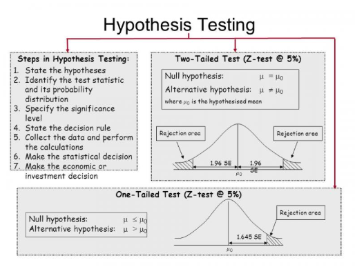
Two-tailed test: Split your alpha level across both ends of the distribution. You are asking: “Is the effect significantly different from zero in either direction?”  One-tailed test: Place your entire alpha at one end. You are asking: “Is the effect significantly larger (or significantly smaller) than zero?”

The One-Tailed Test: When Directionality Is Justified

A one-tailed test is appropriate only when two conditions are simultaneously true. First, you have a specific, theoretically or empirically grounded reason to predict the direction of the effect before seeing the data. Second, a result in the opposite direction would be either impossible, irrelevant, or would be treated the same as a null result.

These conditions are more restrictive than they first appear. They must be satisfied before data collection, not after. Choosing a one-tailed test because your data “suggest” a direction is a form of p-hacking.

Appropriate One-Tailed Examples

• A pharmaceutical company tests whether a new drug reduces blood pressure. It is theoretically implausible that the drug would increase blood pressure, and even if it did, the drug would be rejected. A lower-tailed test is justified.
• An educational intervention is tested to determine whether it improves test scores. There is strong prior evidence from three similar studies that such interventions only ever help, never harm. An upper-tailed test is defensible.
• Engineering: A new alloy is claimed to increase tensile strength. You only care whether it is stronger than the current alloy. Weaker would be equally unacceptable as equal. Upper-tailed test applies.

Inappropriate One-Tailed Examples

• Running a two-tailed test, seeing that results lean in one direction, then switching to a one-tailed test to achieve significance. This is capitalising on chance and inflates Type I error.
• Using a one-tailed test “just to be safe” because you want a lower p-value. One-tailed tests have lower p-values for results in the predicted direction — which is why they are tempting and why they require stronger justification.
• Any exploratory study where you genuinely do not know what direction an effect might take.

The Two-Tailed Test: The Safe Default

When in doubt, use a two-tailed test. This is not a lack of ambition — it is intellectual honesty. Two-tailed tests make no assumption about direction, which makes them appropriate for:

• Any exploratory research where the direction of an effect is unknown or contested
• Situations where an effect in either direction would be meaningful or actionable
• Studies where a surprising reversal of the expected direction would be an important finding in itself
• Essentially all social science research where human behaviour is complex and unpredictable

The cost of using a two-tailed test when a one-tailed test would be justified is modest: you need a slightly larger sample to achieve the same power. The cost of using a one-tailed test when a two-tailed test was appropriate is severe: inflated false-positive rates and potential retraction.

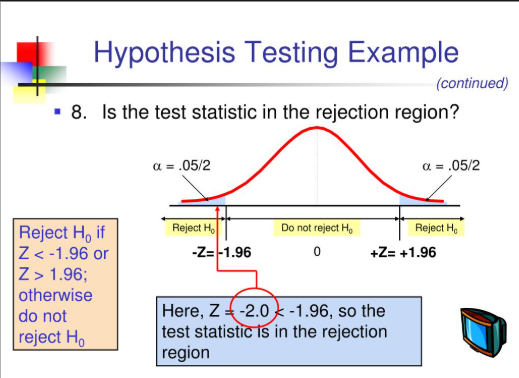
The Numerical Reality: How Much Does the Choice Matter?

For a two-tailed test at alpha = 0.05, you reject the null hypothesis if your t-statistic falls in the most extreme 2.5% at either end of the distribution. For a one-tailed test at alpha = 0.05, you reject if the statistic falls in the most extreme 5% at one end. This means that a one-tailed test is more sensitive to effects in the predicted direction.

Practical translation: A result with p = 0.07 in a two-tailed test might reach p = 0.035 in a one-tailed test — the same data, now technically significant. This is why the choice must be made a priori, not in response to the data.

A Decision Framework You Can Actually Use

Work through these questions in order before running your test:

1. Is there strong prior evidence — from theory, prior literature, or mechanistic reasoning — that the effect can only occur in one direction?
2. Is this prediction documented in your pre-registered analysis plan or thesis proposal, before data collection?
3. Would an effect in the opposite direction truly be of zero scientific or practical interest — treated identically to a null result?

If you answered yes to all three: a one-tailed test is defensible. If you hesitated on any of them: use a two-tailed test and report it transparently.

Reporting Your Choice

Whichever test you use, document your rationale explicitly. Reviewers and readers should never have to guess why a particular test was chosen. A single sentence suffices:

“A one-tailed independent samples t-test was used to assess whether the intervention group scored higher than the control group, consistent with prior literature showing unidirectional effects of this type of intervention (Smith et al., 2021; Jones et al., 2023).”

This kind of transparent reporting signals methodological rigour and protects you from the accusation of post-hoc test selection.

⚡ Key Takeaway:  The safest default in research is always the two-tailed test. Reserve one-tailed tests for situations where prior evidence is strong, the direction is unambiguous, and your decision is pre-registered.

Helping researchers, students, and analysts communicate findings with clarity and confidence.