
Beyond the Randomized Trial: A Step-by-Step Guide to Propensity Score Matching (PSM)
In the world of data analytics and research, the “Gold Standard” is the Randomized Controlled Trial (RCT). By randomly assigning subjects to treatment or control groups, researchers eliminate bias and ensure that any difference in outcomes is due to the treatment itself.
But what happens when you can’t randomize?
Maybe you are a data scientist analyzing the effectiveness of a new marketing campaign where customers self-selected to join. Or a public health researcher evaluating a policy change that only affected certain regions. In observational studies, the treatment group and the control group are often inherently different. If you compare them directly, you are comparing apples to oranges.
Enter Propensity Score Matching (PSM) .
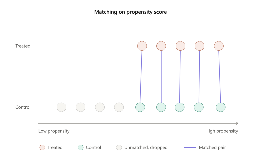
PSM is a statistical technique that mimics the effects of randomization by creating a “quasi-experimental” setup. It allows you to compare treated and untreated subjects who are as similar as possible on observed characteristics.
What is Propensity Score Matching?
At its core, PSM tries to answer the question: “What is the probability that this specific subject would have received the treatment, given their characteristics?”
This probability is the Propensity Score.
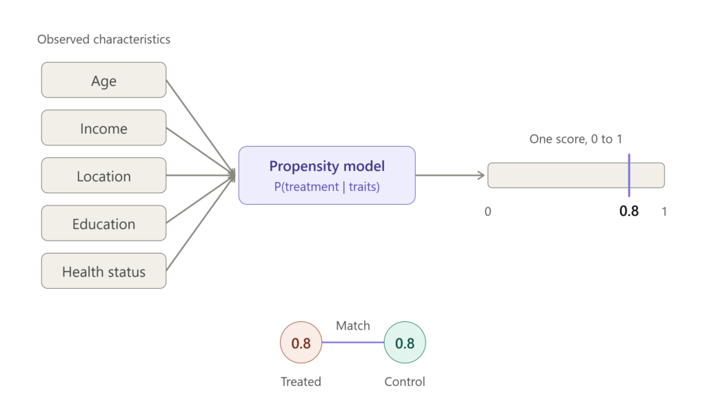
Instead of trying to match subjects on ten different variables (age, income, location, etc.)—which is nearly impossible—PSM collapses all those variables into a single score between 0 and 1. You then match a treated subject with a score of, say, 0.8 to an untreated subject who also has a score of 0.8.
By doing this, you create a control group that looks statistically identical to the treatment group regarding observable traits.
Step 1: Select Covariates (Choose Your Variables)
Before you run any models, you need to choose the variables (covariates) that predict whether a subject receives the treatment.
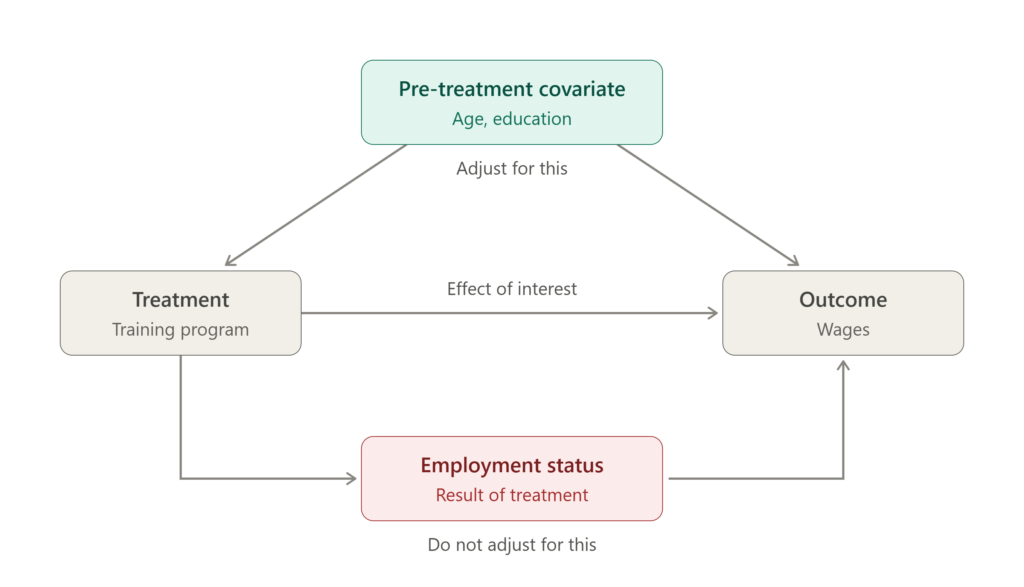
- The Rule of Thumb: Include variables that influence both the treatment assignment and the outcome.
- The Danger: Do not include variables that are purely outcomes of the treatment (post-treatment bias). For example, if you are studying the effect of a job training program on wages, do not include “current employment status” as a covariate if the program helped them get the job.
Step 2: Estimate the Propensity Score
Once you have your variables, you need to calculate the propensity score for every individual in your dataset. The most common method for this is Logistic Regression.
You run a logistic regression where:
- Dependent Variable (Y): Treatment status (1 = Treated, 0 = Control).
- Independent Variables (X): Your selected covariates.
The output gives you the predicted probability (the propensity score) for each subject.
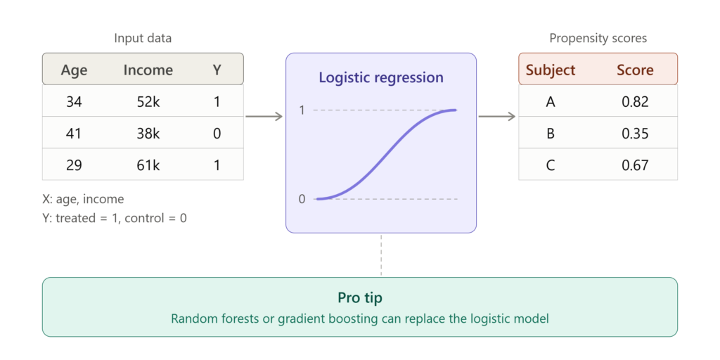
Pro Tip: Some advanced practitioners use Machine Learning (like Random Forests or Gradient Boosting) for this step, as they can capture complex, non-linear relationships better than logistic regression.
Step 3: Perform the Matching
Now that everyone has a score, you need to pair them up. There are several algorithms for this:
- Nearest Neighbor Matching: A treated subject is matched with the control subject who has the closest propensity score.
- Caliper Matching: You set a “tolerance” level. If the nearest neighbor’s score is too far away (e.g., difference > 0.05), the treated subject is discarded because no good match exists.
- Kernel Matching: Instead of matching one-to-one, this uses a weighted average of multiple control subjects to create a match.
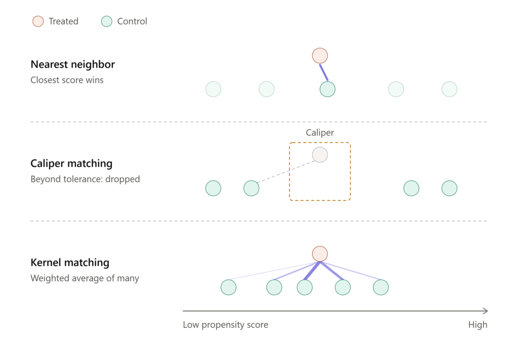
Nearest Neighbor within a Caliper is generally the most popular approach as it balances precision with sample size.
Step 4: Check for Balance (The Most Important Step)
This is where PSM succeeds or fails. You must verify that your matching process actually worked.
You need to check Covariate Balance. Before matching, your treated and control groups likely had significantly different averages (e.g., Treated group average age: 45, Control group average age: 32). After matching, these averages should be nearly identical.
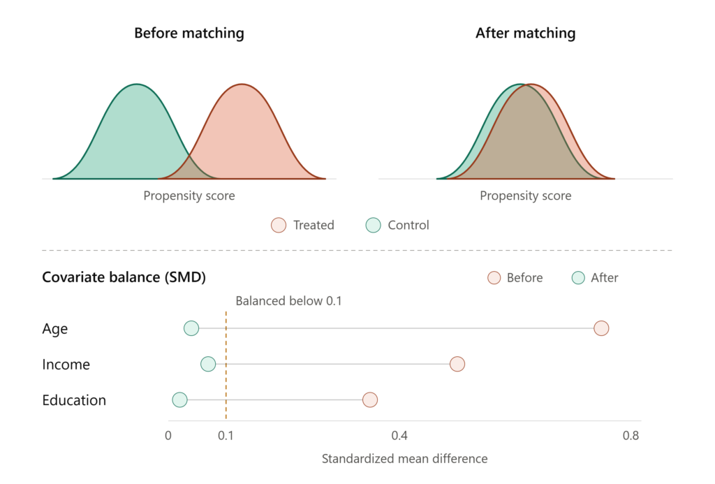
- Standardized Mean Difference (SMD): You want the SMD to be below 0.1 (or 10%) for all covariates after matching.
- Visual Inspection: Use density plots to see if the distribution of propensity scores overlaps between the two groups.
If your data is still unbalanced, you must go back to Step 1 or Step 2 and adjust your model.
Step 5: Estimate the Treatment Effect
Once you have a balanced dataset, you can finally calculate the impact of the treatment. Because you have created a matched sample, you can now compare the outcomes directly.
The metric you are looking for is the Average Treatment Effect on the Treated (ATT) .
[
ATT = \text{Mean Outcome of Treated} – \text{Mean Outcome of Matched Controls}
]
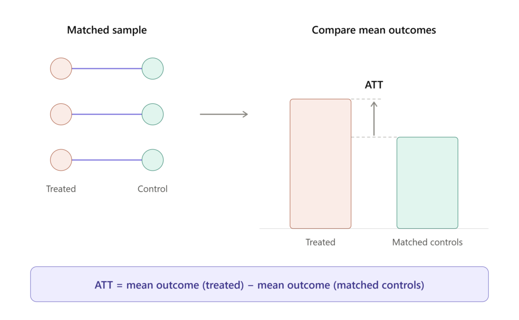
This tells you how much the treatment impacted the group that actually received it.
The Limitations: What PSM Can’t Do
While PSM is powerful, it is not magic. It is crucial to remember its primary limitation: Selection on Observables.
PSM assumes that you have accounted for all the variables that influence both the treatment and the outcome. If there is an unobserved confounder—a variable you didn’t measure (like “motivation” or “genetic predisposition”)—PSM cannot correct for it.
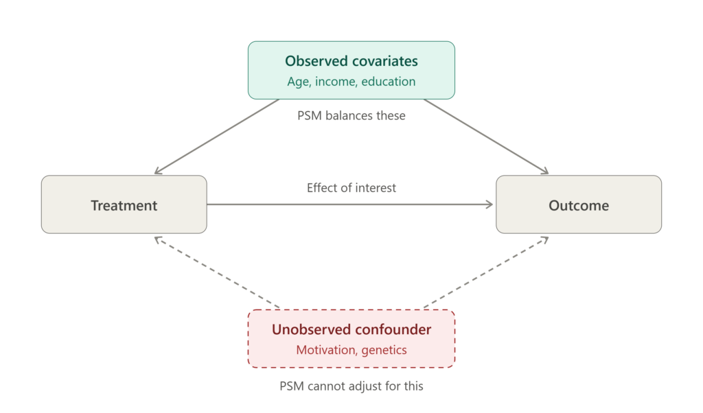
Unlike an RCT, PSM cannot eliminate bias from hidden variables. It only balances the variables you can see.
Conclusion
Propensity Score Matching is a vital tool in the data scientist’s toolkit. It allows us to draw meaningful insights from observational data that would otherwise be too biased to trust. By following these steps—selecting covariates, estimating scores, matching carefully, and checking for balance—you can transform messy observational data into a credible, quasi-experimental study.
Whether you are evaluating social programs, medical treatments, or business strategies, PSM helps you compare apples to apples.
Are you using PSM in your work? What challenges have you faced with covariate selection? Let us know in the comments below!