
Imagine running a four-week A/B test, finding a 2% lift in conversions, and presenting it to your team—only to have a skeptical colleague ask, “Is that real, or just noise?” Without a proper sample size calculation before the experiment begins, you cannot answer that question with confidence. You risk shipping a meaningless change or, worse, abandoning a feature that actually works because your test was too small to detect its effect.
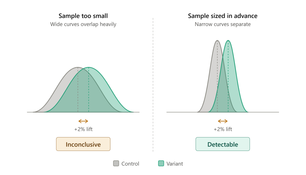
Sample size calculation is the bridge between a vague research question and a statistically credible answer. It forces you to clarify what you are looking for, how precisely you need to measure it, and how much uncertainty you can tolerate. This guide walks through the essential components of sample size calculation for experiments, from the core concepts to practical formulas and common pitfalls.
The Four Inputs You Cannot Skip
Every sample size calculation rests on four parameters. Get these wrong, and your entire experiment inherits the error.
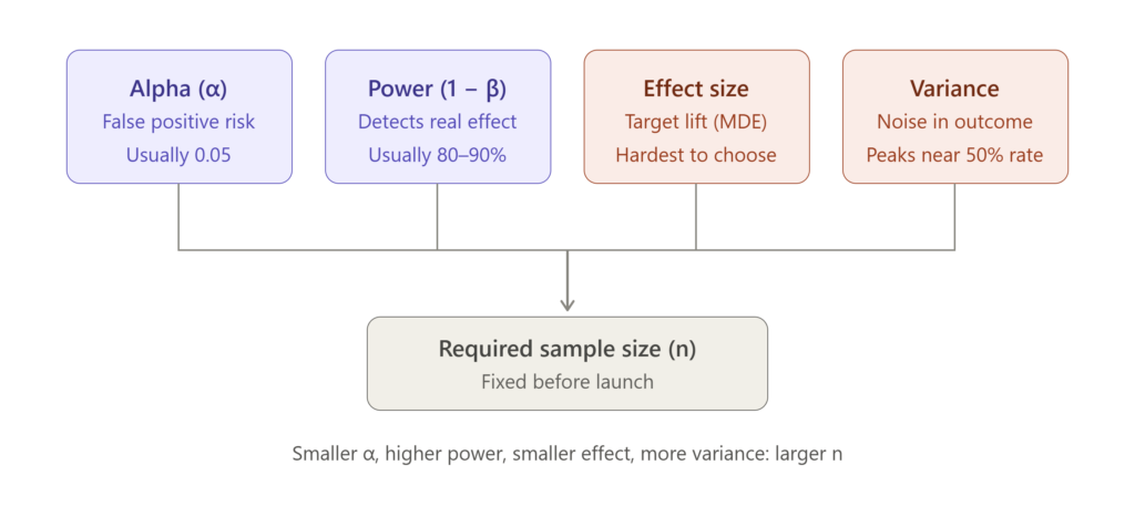
Significance Level (α) is the probability of a false positive—concluding there is an effect when there is none. By convention, researchers set α at 0.05, meaning a 5% risk of a Type I error . For a two-tailed test, this threshold is split across both directions of the effect.
Statistical Power (1 − β) is the probability of detecting an effect if one truly exists. The standard target is 80%, though 90% is preferable for high-stakes decisions . Power and sample size move together: a study powered at 60% has a 40% chance of missing a real effect, which is often unacceptable given the cost of running the experiment.
Effect Size is the magnitude of the difference you want to detect. This is the hardest and most consequential input. You can derive it from prior literature, a pilot study, or a minimum detectable effect (MDE) that represents the smallest change worth caring about commercially. As one methodological primer notes, effect size can be obtained through literature search or calculated from pilot data . If you lack both, you may need to rely on conventional benchmarks—small, medium, large—though these should be treated with caution.
Variance (or Standard Deviation) captures the noise in your outcome variable. For continuous outcomes, the standard deviation determines how many observations you need to distinguish a signal from the background variability. For binary outcomes, variance is a function of the baseline rate: a conversion rate near 50% has maximum variance, while rates near 0% or 100% require fewer samples.
The Core Formula, Demystified
For a comparison of two independent group means, a widely used rule of thumb for the sample size per group is:
n ≈ 8 × (SD / precision)²
where “precision” is the half-width of the confidence interval you want to achieve . This formula assumes equal standard deviations in both groups and gives you roughly a 50% chance of hitting your target precision. For 95% confidence that your interval will be no wider than desired, you need substantially more samples .
For proportions—common in A/B testing—the formula incorporates the baseline rate and the minimum detectable effect. A Python implementation for conversion-rate experiments uses:
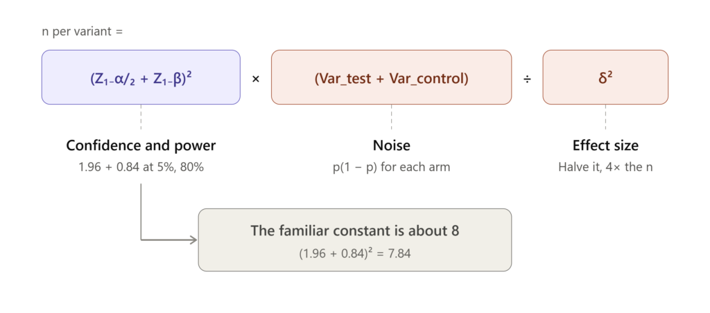
n = (Z₁₋α/₂ + Z₁₋β)² × (Var_test + Var_control) / δ²
where δ is the absolute MDE and the Z-scores correspond to your chosen α and power . Plugging in α = 0.05 (Z ≈ 1.96) and power = 0.80 (Z ≈ 0.84) yields the familiar constants that appear in most online calculators.
The critical insight is that sample size scales with the inverse square of the effect size. Halving the MDE quadruples the required sample. This is why experiments designed to detect tiny effects—common in mature products with small incremental gains—often require hundreds of thousands of observations per variant .
A Worked Example: From Numbers to Decisions
Consider a biomedical researcher planning a study with two independent groups. She wants to detect a medium effect size (Cohen’s d = 0.5) at α = 0.05 with 80% power. Using G*Power, the calculation yields a total sample of 128 participants—64 per group . If she anticipates 10% dropout, she should inflate each group to approximately 71 participants, for a total of 142.
Now consider a paired design, where the same participants are measured before and after an intervention. Because within-subject correlation reduces variability, the required sample is smaller. For a medium within-person effect (dz = 0.5), G*Power recommends 34 participants total—each measured twice . This illustrates a broader principle: design efficiency matters as much as raw sample size. Paired designs, stratified sampling, and covariate adjustment can all reduce the number of observations needed by shrinking the unexplained variance.
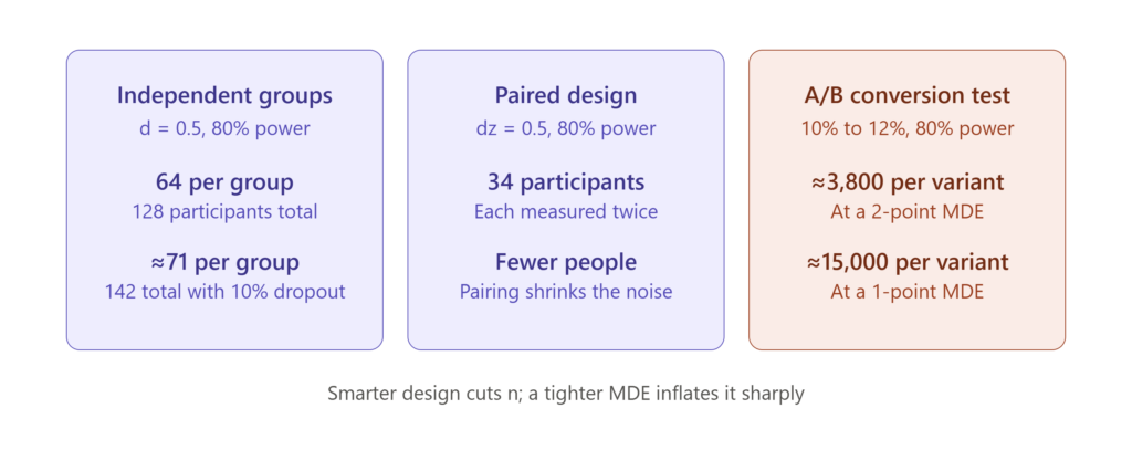
For a proportional outcome, suppose a product team wants to detect a lift from 10% to 12% in conversion rate (an absolute MDE of 2 percentage points). With α = 0.05 and 80% power, a standard A/B test calculator would return roughly 3,800 users per variant. If the team can only tolerate a 1-point MDE, the requirement jumps to approximately 15,000 per variant. This nonlinearity is why defining the MDE honestly—rather than optimistically—is essential.
What Most People Get Wrong
Ignoring the MDE trap. Teams often calculate sample size based on the effect they hope to see rather than the smallest effect they need to detect. If the true effect is smaller than the MDE, the experiment will be underpowered and may produce a false negative. Always ask: what is the minimum change that would actually change our decision? That is your MDE.
Forgetting dropout and data quality. A calculated sample of 500 per group means 500 usable observations. Attrition, bot traffic, incomplete responses, and exclusion criteria all erode your effective sample. Inflate your target by 10–20% to account for these losses .
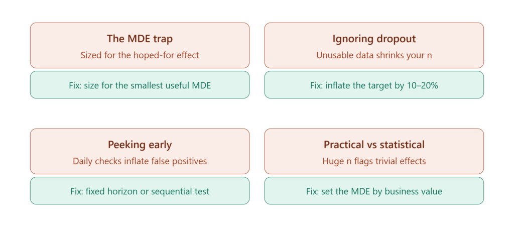
Peeking and stopping early. Sample size calculations assume a fixed sample analyzed once. If you check results daily and stop when the p-value crosses 0.05, your false positive rate inflates dramatically. Sequential testing methods exist, but they require different sample size formulas .
Confusing statistical and practical significance. A massive sample can make a trivial effect statistically significant. A sample size calculated for a meaningful MDE protects against this—if the effect is too small to matter, the experiment is designed not to detect it as significant.
Tools and Reporting
For most researchers, dedicated software is more reliable than hand calculations. G*Power is free and widely used in the social and biomedical sciences, with templates for t-tests, ANOVA, correlation, and regression . R packages and Python libraries offer programmatic alternatives for analysts who want reproducible pipelines .
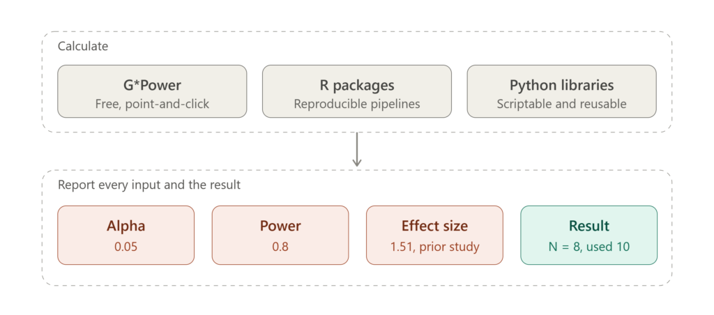
When reporting your calculation, be explicit about all four inputs. A rigorous example from a published paper states: “The effect size in prior study was 1.51. With a significance criterion of α = 0.05 and power = 0.8, the minimum sample size per group needed with this effect size is N = 8. Therefore, sample size of N = 10 per group was obtained” . This transparency allows reviewers and collaborators to evaluate whether your assumptions were reasonable.
The Bottom Line
Sample size calculation is not a bureaucratic hurdle—it is the moment when you confront whether your experiment can actually answer the question you are asking. A study that is too small wastes resources and produces ambiguous results. A study that is unnecessarily large wastes time and may expose participants to risk without added benefit. The calculation forces precision in your thinking: What effect matters? How much noise must I overcome? What error rates can I tolerate?
Run the numbers before you collect a single data point. Your future self—and anyone who relies on your results—will thank you.